Approx TSP Tour

Is an Approximation Algorithm that assumes the Triangle Inequality for solving the Traveling Salesman Problem with an Approximation Ratio of 2.

Pseudocode

def approx_TSP_tour(G, c):
    # Select a root vertex (using vertex 0 as default)
    r = 0
 
    # Compute MST using Prim's algorithm
    T = MST_PRIM(G, c, r)
 
    # Perform preorder traversal of the MST
    H = preorder_traversal(T, r, [])
 
    return H
 
 
 def preorder_traversal(tree, vertex, visited):
        if vertex not in visited:
            visited.append(vertex)
            for neighbor in tree[vertex]:
                preorder_traversal(tree, neighbor, visited)
        return visited

The code use Prim’s Algorithm to construct a Minimum Spanning Tree and afterwards does a preorder walk.

A preorder tree walk is performed by starting at the root, and performing the following recursively:

1. Visit the root.
2. Visit the left sub-tree of the root.
3. Visit the right sub-tree of the root.

The preorder_traversal returns the nodes in the order that they were first visited using the preorder tree walk.

Theorems

Approximation Ratio and runtime

Approx TSP Tour is a polynomial-time 2-approximation algorithm for the Traveling Salesman Problem with the Triangle Inequality.

Proof

See CLRS p.1114

Examples

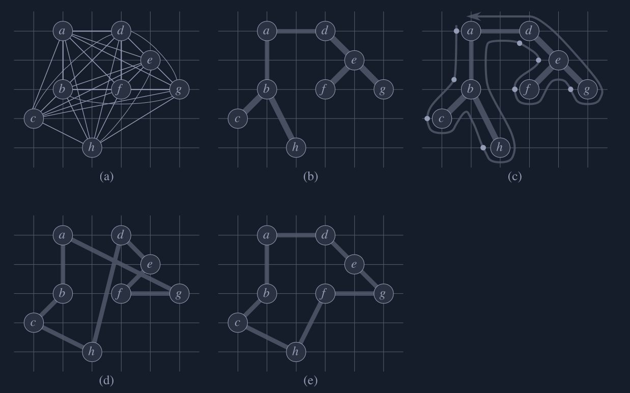(a) A complete undirected graph. Vertices lie on intersections of integer grid lines. For example, $f$ is one unit to the right and two units up from $h$. The cost function between two points is the ordinary euclidean distance.

(b) A minimum spanning tree $T$ of the complete graph, as computed by MST-PRIM. Vertex $a$ is the root vertex. Only edges in the minimum spanning tree are shown. The vertices happen to be labeled in such a way that they are added to the main tree by MST-PRIM in alphabetical order.

(c) A walk of $T$, starting at $a$. A full walk of the tree visits the vertices in the order $a,b,c,b,h,b,a,d,e,f,e,g,e,d,a$. A preorder walk of $T$ lists a vertex just when it is first encountered, as indicated by the dot next to each vertex, yielding the ordering $a,b,c,h,d,e,f,g$.

(d) A tour obtained by visiting the vertices in the order given by the preorder walk, which is the tour $H$ returned by APPROX-TSP-TOUR. Its total cost is approximately $19.074$.

(e) An optimal tour $H^{\text{*}}$ for the original complete graph. Its total cost is approximately $14.715$.