The Distance-Vector (DV) Routing Algorithm

A Decentralised Routing Algorithm that constructs a forwarding table in each node by having nodes propagate information to their neighbours.

The algorithm is:

• Distributed: Each node in a graph receives information from their neighbours, performs a computation and distributes the results to their neighbours.
• Iterative: The process continues until no more information is exchanged at which point the nodes will have learned the least-cost paths from them-self to other nodes.
• Asynchronous: Since the nodes need not operate in lockstep with each other.

The information distributed for each node $x$ in the graph $N$ is their distance-vector ${\mathbf{D}}_x=[D_x(y):y\in N]$ where $D_x(y)$ is an estimate of the least-cost path from $x$ to $y$. The distance vector is therefore a vector of least cost paths to other nodes in the network.

Each node $x$ maintains the following information:

• For each neighbour $v$, the cost $(x,v)$ from $x$ directly attached to $v$.
• Node $x$‘s distance vector ${\mathbf{D}}_x$.
• The distance vectors of its neighbours ${\mathbf{D}}_v$.

This distance vector is computed when receiving other neighbours distance vectors by using the The Bellman-Ford Equation. If this results in their distance-vector changing, then they broadcast their updated distance-vectors to neighbours. The same is done if a node experiences a change in its attached links.

As long as the nodes keep exchanging their distance-vectors then the least-cost estimates $D_x(y)$ will converge to the actual least-cost estimate $d_x(y)$ according to Bertsekas 1991.

Pseudo code

Runs at each node x:

 
# ─────────────────────────────────────────
# INITIALISATION
# ─────────────────────────────────────────
for y in N:  # all destinations
    Dx[y] = c(x, y)  # cost to neighbour; infinity if y is not a neighbour
 
for w in neighbours(x):
    Dw[y] = float('inf') for all y in N  # neighbour costs unknown initially
 
for w in neighbours(x):
    send(Dx, to=w)  # send own distance vector Dx = {y: Dx[y] for y in N} to w
 
# ─────────────────────────────────────────
# MAIN LOOP
# ─────────────────────────────────────────
while True:
    # Wait for a trigger
    wait until (
        link_cost_changed(to_neighbour=w)
        or received_distance_vector(from_neighbour=w)
    )
 
    # Recompute distances using Bellman-Ford
    for y in N:
        Dx[y] = min(c(x, v) + Dv[y] for v in neighbours(x))
 
    # Propagate updates if anything changed
    if any(Dx[y] changed for y in N):
        for w in neighbours(x):
            send(Dx, to=w)  # send Dx = {y: Dx[y] for y in N} to all neighbours

Count-to-infinity Problem

Is a problem where many (not infinity but an unbounded value) iterations are needed to properly update the distance vectors as a result of an increase in link cost.

Se examples for demonstration.

Poisoned reverse

The three node example of the count-to-infinity problem can be avoided by the poisoned reverse technique. This works by having nodes that route through other nodes to a third node advertise a cost of infinity to the intermediary node, i.e. if $z$ routes through $y$ on its way to $x$ then $z$ informs $y$ that $D_z(x)=\infty$.

This however does not solve the count-to-infinity problem when the loop contains three or more nodes.

Examples

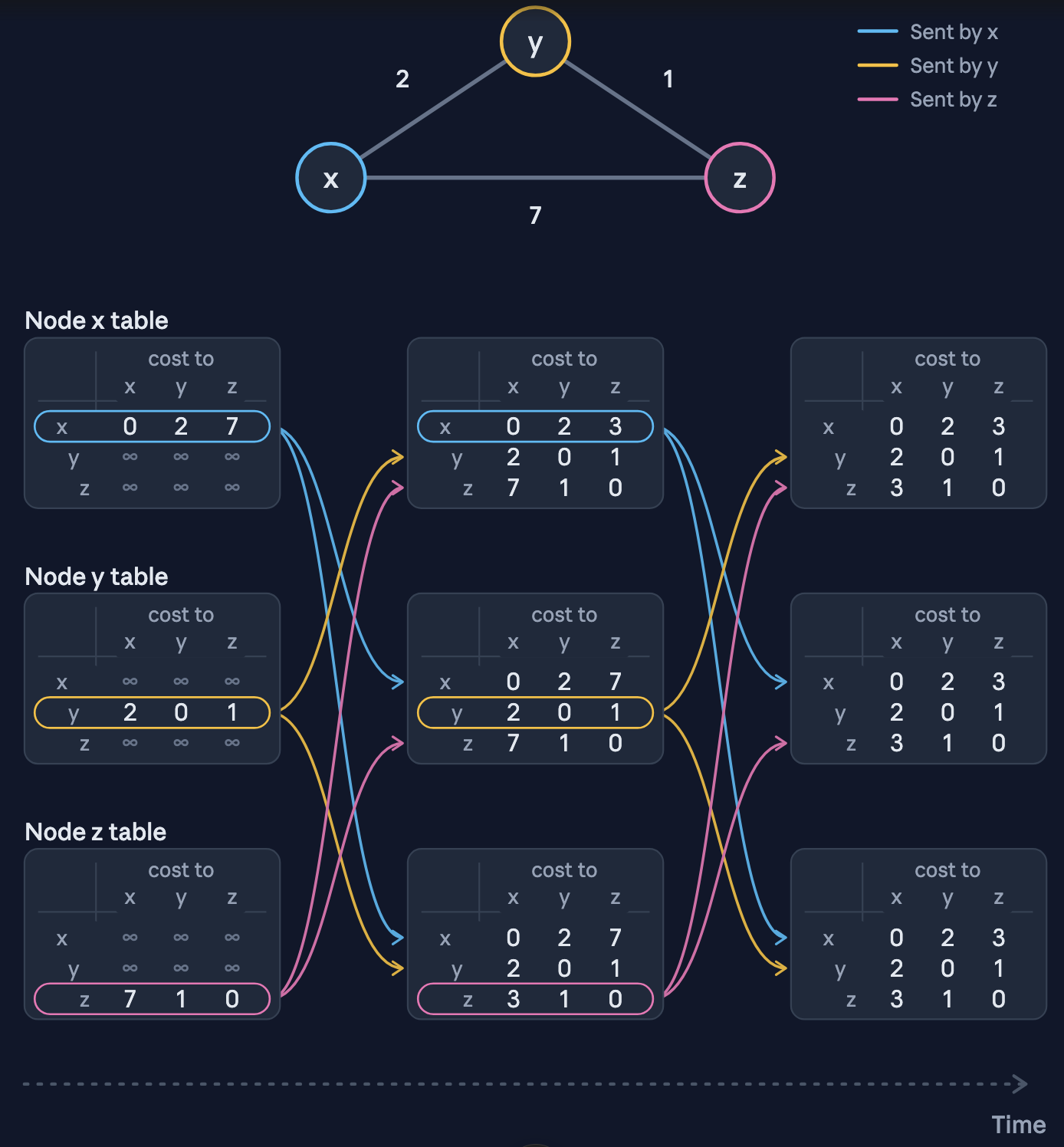
Three node graph

Count-to-infinity Problem

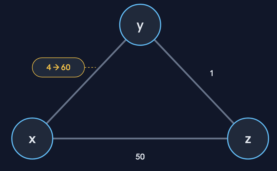$c(x,y)$ is changed from 4 to 60.

Before change

Before the link cost is changed we have $D_y(x)=4,D_y(z)=1,D_z(5)$.

t0: Change is discovered

$y$ detects link change and computes $$\begin{gathered} D_y(x)=\min \\ c(y,x)+D_x(x),c(y,z)+D_z(x) \\ =\min \\ 60+0,1+5 \\ =6 \end{gathered}$$ Of course we know that $D_z(x)$ should be 50 but $z$ has not yet gained this information.

t1: y inform z of new cost

Node $y$ has computed a new cost to $x$ and informs $z$ of this change.

$z$ then use this new information to compute $$\begin{gathered} D_z(x)=\min \\ c(z,x)+D_z(z),c(z,y)+D_y(x) \\ =\min \\ 50+0,1+6 \\ =7 \end{gathered}$$

t2: z inform y of new cost

Since node $z$ has updated its new cost to $x$ it informs $y$ of this change and $y$ computes $D_y(x)=8$.

t3: y informs z of new cost

Since $y$ has updated its new cost to $x$ it informs $z$. This pattern repeats until $y$ and $z$, where they increment their cost to $x$ by one, until they have reached $D_z(x)=50$ and $D_y(x)=51$, which are the true least costs.