Recurrent Neural Networks (RNNs)

Neural networks that, contrary to Feedforward Neural Networks, contains a cycle, meaning that the value of some unit is either directly or indirectly dependant on its own earlier outputs as an input. This enables RNNs to detect temporal patterns within sequences.

Architecture

The term RNN is used for any network with recurrent properties, but here we focus on simple recurrent networks or Elman Networks (Elman 1990). These have three type of layers: input, hidden and output. The hidden layer is connected to the input, itself, and output layers as seen below. 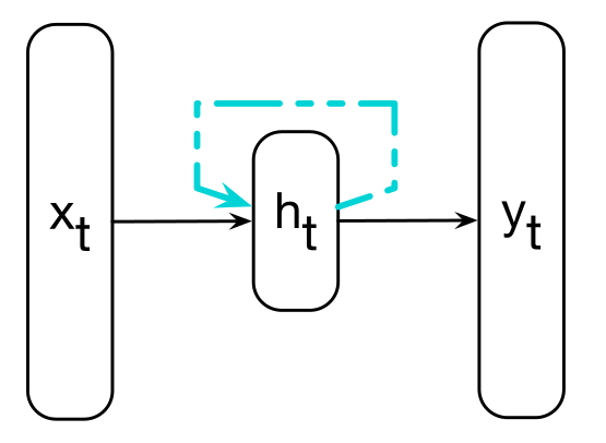It stores information about the context by sending activation values back to itself over several steps, one for each input value fed into the network. This feedback loop is what make the inputs have effect on each other, and is also the only reason for making calculations for these inputs as only the output layer of the final input is used.

Thus, to compute an output ${\mathbf{y}}_t$ for an input ${\mathbf{x}}_t$ we need the activation value for the hidden layer ${\mathbf{h}}_t$ and thus calculate it as follows ${\mathbf{h}}_t=g(\mathbf{W}{\mathbf{x}}_t+\mathbf{U}{h}_{t-1})$ ${\mathbf{y}}_t=f(\mathbf{V}{\mathbf{h}}_t)$ where $f$ and $g$ are activation functions, and $\mathbf{W},\mathbf{U}$, and $\mathbf{V}$ are weight matrices. Thus to compute ${\mathbf{y}}_n$ for a sequence ${\mathbf{x}}_1,{\mathbf{x}}_2,\dots ,{\mathbf{x}}_n$ we do not need to compute ${\mathbf{y}}_1,{\mathbf{y}}_2,\dots ,{\mathbf{y}}_{n-1}$ as these inputs are only needed to calculate ${\mathbf{h}}_1,{\mathbf{h}}_2,\dots ,{\mathbf{h}}_n$.

Training

To train using Backpropagation one now needs to asses how much ${\mathbf{h}}_t$ contributes to loss by knowing its influence on both ${\mathbf{y}}_t$ and ${\mathbf{y}}_{t+1}$. This is done with Backpropagation Through Time (Werbos 1990), which first does a forward pass that computes ${\mathbf{h}}_t$ and ${\mathbf{y}}_t$ and accumulate the loss at each step of the sequence, saving the value of the hidden layer at each step for use at the next step. The next phase process the sequence in reverse and computes the required gradients as it goes and saves the error term for use in the hidden layer for each step back in time.

This approach can be seen as unrolling the RNN into a Feedforward Neural Networks, as shown below, and doing normal Backpropagation. 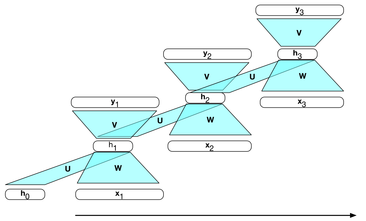This removes any explicit recurrence and allows the weights to be trained directly. These weights however are shared across all time steps.